Scheduling Problem in HPC Systems

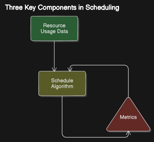
Job scheduling is a critical aspect of high-performance computing (HPC) systems, where multiple tasks or jobs need to be allocated to available resources in an efficient and optimal manner. The goal of job scheduling is to maximize system utilization, minimize job completion times, and ensure fair allocation of resources to different users or applications. In simplified terms, this challenge involves developing three key components, like this figure shows:

Background

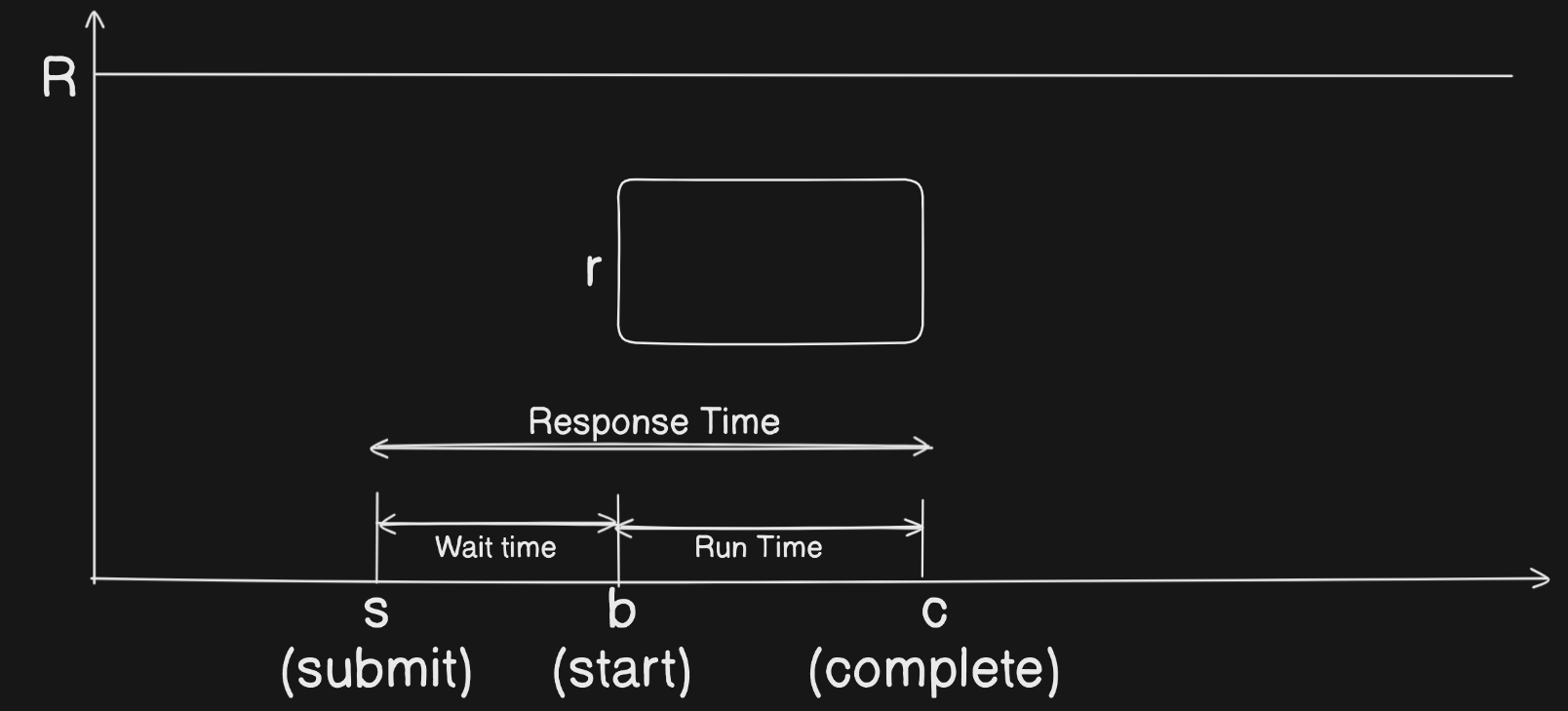
The following diagram of job lifecycle in HPC systems shows the different stages of a job from submission to completion:

Formally, jobs are arriving at the system at their submit time $s_i$. After that, they are queued in the system until they are scheduled to run on the available resources. Once a job is scheduled, it starts executing on the allocated resources at its start time $b_i$. The time it takes to wait in the queue is waiting time $Q_i$:

$$Q_i = b_i - s_i$$

After the job starts, it executes for the duration of its runtime $D_i$ and finishes at completion time $c_i$:

$$D_i =c_i − b_i.$$

The total time a job spends in the system is the turnaround time $F_i$:

$$F_i = c_i − s_i = Q_i + D_i.$$

The job using resources during its runtime as shown in the following equation:

$$r_j(t) = \begin{cases} r_j, & \text{if } b_j \leq t < c_j \\ 0, & \text{otherwise} \end{cases}$$

and assuming the total amount of resources in the cluster is 𝑅, the following constraint applies:

$$\forall t : \sum_{j \in J} r_j(t) \leq R$$

Where:

t represents a moment in time.

J is the set of jobs in the schedule.

Metrics for Scheduling

Average Response Time (AF)

The average response time $AF(J)$ is given by:

$$AF(J) = \frac{1}{|J|} \sum_{j \in J} F_j$$

where J represents the set of jobs in the schedule.

This metric measures the average time a job spends in the system from submission to completion. A lower average response time indicates better performance in terms of job completion times.

Average Bounded Slowdown (BSLD)

The average bounded slowdown $BSLD(J)$ is given by:

$$BSLD(J) = \frac{1}{|J|} \sum_{j \in J} \max \left( 1, \frac{F_j}{\max(D_j, k)} \right)$$

where $k$ is a lower bound

This is a common metric in HPC job scheduling, calculated as the ratio of response time to runtime. Since very short jobs can disproportionately affect the Average Slowdown.

Although adding $k$ helps limit the impact of short jobs, it can also have negative effects. For jobs where $D_j < k < F_j$, BSLD reverts to the Average Flow Time (AF), and jobs with response times below $k$ no longer contribute to the metric.

Area-Weighted average Response Time (AWF)

In HPC job scheduling, Area-Weighted Response Time (AWF) is a key metric used to assess packing efficiency. AWF minimizes the weighted sum of job completion times, with job weights representing the "effort" required, often referred to as the "area" (resource usage × runtime).

AWF has several advantages:

1. Starting a job earlier while keeping other start times unchanged reduces AWF.
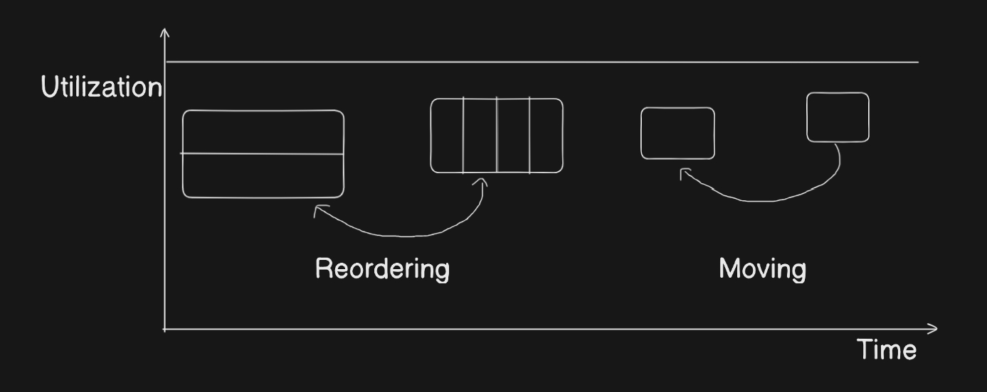
2. Reordering jobs without changing the resource usage profile doesn’t affect AWF.
3. Dividing or combining jobs (while keeping the resource usage unchanged) doesn’t impact AWF.

The Area-Weighted Response Time (AWF) is given by:

$$AWF(J) = \frac{\sum_{j \in J} r_j D_j F_j}{\sum_{j \in J} r_j D_j}$$

Level-α Priority Weighted Specific Response Time (PαSF)

When referring to job priorities, we can imply two rather different concepts:

1. Priority based on job usefulness: This type of priority reflects a job’s code efficiency or the importance of its associated project. In this case, the weights in the Area-Weighted average Response Time (AWF) can be modified as $w_j = p_j r_j D_j$, where $p_j$ represents the priority of job $j$. This adjustment is simple and does not require further elaboration.

2. Priority based on fairness: Here, the focus shifts to the idea that jobs which have waited longer should be prioritized. To maintain the new metric's independence from job size, we propose a method where jobs are composed of infinitesimal "units of computation," each requiring $dr$ resources and $dt$ running time. The Level-α Priority Weighted Specific Response Time (PαSF) metric, defined as:

$$PαSF(J) = \frac{\alpha + 1}{\alpha + 2} \cdot \frac{\sum r_j (F_j^{\alpha + 2} - Q_j^{\alpha + 2})}{\sum r_j (F_j^{\alpha + 1} - Q_j^{\alpha + 1})},$$

balances fairness and packing efficiency. The parameter $\alpha$ controls this balance, with larger values of $\alpha$ giving more weight to fairness. A reasonable range for $\alpha$ is between 1 and 3, as values greater than 3 may disproportionately emphasize poorly scheduled jobs and reduce the metric's overall responsiveness.

PαSF, alongside AWF, offers a nuanced perspective for evaluating scheduling algorithms, revealing advantages and drawbacks that traditional metrics like BSLD often miss.

Loss of Capacity (LoC)

Another metric suggested to measure job packing is Loss of Capacity (LOC)

$$LOC = \frac{ \int_{\min\limits_{1 \leq j \leq n} (s_j)}^{\max\limits_{1 \leq j \leq n} (c_j)} \min (\sum\limits_{j : s_j < t < b_j} r_j, R - \sum\limits_{j : b_j < t < c_j} r_j) dt }{ (\max\limits_{1 \leq j \leq n} (c_j) - \min\limits_{1 \leq j \leq n} (s_j)) \times R }$$

where:
- $ R $ is the total number of nodes in the cluster.
- $ c_j $ is the completion time of job $ j $.
- $ s_j $ is the start time of job $ j $.
- $ r_j $ is the resource usage of job $ j $.

Some Scheduling Algorithms

First-Come, First-Served (FCFS)

First-Come, First-Served (FCFS) is one of the simplest scheduling algorithms in scheduling. In FCFS, the process that arrives first is executed first. Processes are executed in the order they enter the queue, with no prioritization. This algorithm is easy to understand and implement but can lead to long waiting times for high-priority jobs.

Example:

Assume the following jobs arrive at the system:

Job 1: Arrival Time = 0, Required CPU Time = 5
Job 2: Arrival Time = 1, Required CPU Time = 3
Job 3: Arrival Time = 2, Required CPU Time = 1

FCFS Scheduling:

Job 1: 0 - 5
Job 2: 5 - 8
Job 3: 8 - 9

Even though Process C requires only 1 second, it must wait until both Process A and B finish, showing how FCFS can lead to delays for shorter processes.

Shortest Job First (SJF)

Shortest Job First (SJF) is a scheduling algorithm that selects the process with the smallest execution time. This algorithm minimizes the average waiting time for all processes. SJF is a non-preemptive algorithm, meaning that once a process starts executing, it continues until completion. If a new process arrives with a shorter execution time than the current process, the current process is preempted and the new process is executed.

Example:

Assume the following jobs arrive at the system:

Job 1: Arrival Time = 0, Required CPU Time = 5
Job 2: Arrival Time = 1, Required CPU Time = 3
Job 3: Arrival Time = 2, Required CPU Time = 1

SJF Scheduling:

Job 3: 0 - 1
Job 2: 1 - 4
Job 1: 4 - 9

In this example, the SJF algorithm schedules the shortest job first, resulting in a more efficient use of resources and reduced waiting times.

EASY Backfilling

EASY Backfilling is a scheduling algorithm that aims to improve the efficiency of job scheduling in HPC systems. In EASY Backfilling, jobs are scheduled in a first-come, first-served (FCFS) manner, but the scheduler can backfill idle slots with shorter jobs that can be completed before the next scheduled job. This allows the system to make better use of available resources and reduce job waiting times.

Example:

Assume the following jobs arrive at the system:

Job 1: Arrival Time = 0, Required CPU Time = 5
Job 2: Arrival Time = 1, Required CPU Time = 3
Job 3: Arrival Time = 2, Required CPU Time = 1

EASY Backfilling Scheduling:

Job 1: 0 - 5
Job 3: 5 - 6
Job 2: 6 - 9

Round Robin (RR)

Round Robin (RR) is a scheduling algorithm that assigns a fixed time slice to each process in the queue. Once a process's time slice expires, it is moved to the back of the queue, and the next process is executed. RR is a preemptive algorithm that ensures all processes get an equal share of the CPU time. If a process's execution time exceeds the time slice, it is moved to the back of the queue and the next process is executed

Example:

Assume the following jobs arrive at the system:

Job 1: Arrival Time = 0, Required CPU Time = 5
Job 2: Arrival Time = 1, Required CPU Time = 3
Job 3: Arrival Time = 2, Required CPU Time = 1

Round Robin Scheduling (Time Slice = 2):

Job 1: 0 - 2
Job 2: 2 - 4
Job 3: 4 - 5
Job 1: 5 - 7
Job 2: 7 - 9

Simulation of Scheduling in HPC Systems by pybatsim