Reinforcement Learning

Introduction to Reinforcement Learning

Reinforcement learning is a type of machine learning that involves training an agent to interact with an environment and learn the best actions to take in different situations. The agent receives feedback in the form of rewards or penalties based on its actions, and its goal is to maximize the total reward it receives over time. Reinforcement learning is inspired by the way humans and animals learn from trial and error, and it has been successfully applied to a wide range of problems, including game playing, robotics, and resource allocation.

Background

Reinforcement learning is based on the idea of an agent interacting with an environment to learn the best actions to take in different situations. The agent receives feedback in the form of rewards or penalties based on its actions, and its goal is to maximize the total reward it receives over time. The agent learns by exploring the environment and trying different actions, and it uses the feedback it receives to update its policy or strategy for choosing actions.

Reinforcement Learning Components

Agent: The entity that interacts with the environment and learns to take actions to maximize its reward.

Environment: the external world that the agent interacts with and receives feedback from.

State: A representation of the current situation or context in which the agent finds itself.

Action: A transposable decision that the agent can take in a given state.

Reward: A scalar value that the agent receives from the environment after taking an action in a given state.

Policy: A mapping from states to actions that the agent uses to make decisions.

Value Function: A function that estimates the expected total reward the agent will receive from a given state.

Model: A representation of the environment that the agent uses to predict the next state and reward based on its current state and action.

Exploration vs. Exploitation in RL

Exploration is the process of trying out new actions to gain information about the environment. It allows the agent to discover new states and learn how to behave in those states. However, excessive exploration may prevent the agent from exploiting its current knowledge of the environment.

Exploitation is the process of taking actions that the agent believes will maximize its expected cumulative reward based on its current knowledge of the environment. It allows the agent to maximize its reward in the short term. However, excessive exploitation may prevent the agent from discovering better policies.

To find an optimal policy, the agent must balance exploration and exploitation. It must explore enough to discover new states and actions, but also exploit enough to take actions that maximize its expected cumulative reward

Solution for Trade-off:

• Epsilon-Greedy Policy: The agent chooses a random action with probability epsilon and the best action with probability 1-epsilon.

• Softmax Policy: The agent chooses actions probabilistically based on their estimated values.

• Upper Confidence Bound (UCB): The agent chooses actions based on their estimated values and a measure of uncertainty.

Reinforcement Learning Algorithms

Tabular Solution Methods

1. Markov Decision Process (MDP)

Markov State: A state in which the future state depends only on the current state and action.

Example:

	Rainy	Cloudy	Sunny
Rainy	0.3	0.4	0.3
Cloudy	0.2	0.6	0.2
Sunny	0.1	0.2	0.7

MDP MDP provides a mathematical framework for modeling decision-making problems in which an agent interacts with an environment over time.

Contain

• Possible states of the environment
• Possible actions the agent can take
• Rewards function
• Transition probabilities

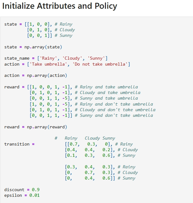
Demo for MDP: MDP Demo

With these parameters below:

Across the MDP, the agent can take actions to move from one state to another. The agent receives a reward for each action it takes, and its goal is to maximize the total reward it receives over time:

Discount Factor: A discount factor is used to discount future rewards relative to immediate rewards. It is used to ensure that the agent values immediate rewards more than future rewards. It is denoted by the symbol gamma (γ) and is a value between 0 and 1.

Example:

• If the discount factor is 0, the agent only cares about immediate rewards.
• If the discount factor is 1, the agent values all rewards equally.
• If the discount factor is between 0 and 1, the agent values immediate rewards more than future rewards.

Bellman Equation

They share the same state-value function, called the optimal state-value function, denoted $v_*$, and defined as:

$v_*(s) = \max_{\pi} v_{\pi}(s) \ \ \ \forall s \in S$

Optimal action-value function, denoted q , and defined as:

$q_*(s, a) = \max_{\pi} q_{\pi}(s, a) \ \ \ \forall s \in S, a \in A$

Thus, we can write q in terms of v as follows:

$q_*(s, a) = \mathbb{E}[R_{t+1} + γv_*(S_{t+1}) | S_t = s, A_t = a]$

Because it is the optimal value function, the consistency condition for $v$ can be written in a special form without reference to any specific policy. This is the Bellman equation for $v$, or the Bellman optimality equation. Intuitively, the Bellman optimality equation expresses the fact that the value of a state under an optimal policy must equal the expected return for the best action from that state:

$$v_*(s) = \max_{a \in A(s)} {q_\pi}_*(s, a)$$ $$= \max_{a} \mathbb{E_\pi*} \left[G_t \mid S_t = s, A_t = a \right]$$ $$= \max_{a} \mathbb{E_\pi*} \left[ \sum_{k=0}^{\infty} R_{t+k+1} \mid S_t = s, A_t = a \right]$$ $$= \max_{a} \mathbb{E_\pi*} \left[ R_{t+1} + γ\sum_{k=0}^{\infty} γR_{t+k+2} \mid S_t = s, A_t = a \right]$$ $$= \max_{a} \mathbb{E} \left[ R_{t+1} + γv_*(S_{t+1}) \mid S_t = s, A_t = a \right]$$ $$= \max_{a \in A(s)} \sum_{s', r} p(s', r \mid s, a) \left( r + γv_*(s') \right)$$

Hai biểu thức cuối cùng là hai dạng chuẩn tắc của phương trình Bellman tối ưu cho $v$. Phương trình Bellman tối ưu cho $q$ là:

$$q_*(s, a) = \mathbb{E} \left[ R_{t+1} + γ \max_{a'} q_*(S_{t+1}, a') \mid S_t = s, A_t = a \right]$$ $$= \sum_{s', r} p(s', r \mid s, a) \left( r + γ \max_{a'} q_*(s', a') \right)$$

Demo for Bellman Equation: Bellman Equation

2. Monte Carlo Methods

3. Dynamic Programming

4. Temporal Difference Learning

Approximate Solution Methods

1. Value Prediction with Function Approximation

2. Gradient-Descent Methods

3. Linear Methods

Q-Learning

Deep Learning

Deep Q-Networks (DQN)

Double Deep Q Networks (DDQN)

Reinforcement Learning in Practice

Conclusion