Derivatives of all layers

Derivatives with Respect to Individual Parameters

In feedforward step For a given input value x$`, the output of the neural network is computed. During this computation, the activations$a^l$ at each layer are stored for later use.

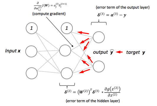
For each unit j in the output layer, compute the error term:

$$e^{L}_j = \frac{\partial J}{\partial z^{L}_j}$$

From this, we can derive the following:

$$\frac{\partial J}{\partial w^{L}_{ij}} = a^{L-1}_i e^{L}_j$$ $$\frac{\partial J}{\partial b^{L}_j} = e^{L}_j$$

For layers $l = L-1, L-2, \ldots, 1$, we compute:

$$e^{l}_j = \left( w^{l+1}_j : e^{l+1} \right) f'(z^{l}_j)$$

Updating the derivatives for each parameter yields:

$$\frac{\partial J}{\partial w^{l}_{ij}} = a^{l-1}_i e^{l}_j$$ $$\frac{\partial J}{\partial b^{l}_j} = e^{l}_j$$

Derivatives with Respect to Matrices

The computation of derivatives for individual parameters as described above is useful for understanding the principles involved. However, in practice, we need to optimize the calculations by expressing them in vector and matrix forms to accelerate the algorithm. Let’s define:

$$e^{l} = \begin{bmatrix} e^{l}_1 \\ e^{l}_2 \\ \vdots \\ e^{l}_{d^{l}} \end{bmatrix} \in \mathbb{R}^{d^{l} \times 1}$$

Feedforward Step: For a given input value $x$, compute the network output while storing the activations $a^{l}$ at each layer.

For the output layer, compute:

$$e^{L} = \frac{\partial J}{\partial z^{L}}$$

From this, we deduce:

$$\frac{\partial J}{\partial W^{L}} = a^{L-1} (e^{L})^T$$ $$\frac{\partial J}{\partial b^{L}} = e^{L}$$

For layers $l = L-1, L-2, \ldots, 1$:

$$e^{l} = \left( W^{l+1} e^{l+1} \right) \odot f'(z^{l})$$

Here, $\odot$ denotes the element-wise product (Hadamard product), meaning each component of the two vectors is multiplied together to yield a resultant vector.

Updating the Derivatives for the Weight Matrices and Bias Vectors

$$\frac{\partial J}{\partial W^{l}} = a^{l-1} (e^{l})^T$$ $$\frac{\partial J}{\partial b^{l}} = e^{l}$$

Note: The expression for the derivative in the previous line might raise a question: why is it $a^{L-1} (e^{L})^T$ and not $a^{L-1T} e^{L}$ or others? A key rule to remember is that the dimensions of the two matrices on the right-hand side must match. Testing this reveals that the left-hand side represents the derivative with respect to $W^{L}$, which has a dimension $\mathbb{R}^{d^{L-1} \times d^{L}}$. Thus, $e^{L} \in \mathbb{R}^{d^{L} \times 1}$ and $a^{L-1} \in \mathbb{R}^{d^{L-1} \times 1}$ imply that the correct formulation must be $a^{L-1} (e^{L})^T$. Additionally, the derivative with respect to a matrix of a scalar-valued function will have dimensions matching that of the matrix.

Backpropagation for Batch (Mini-Batch) Gradient Descent

What happens when we want to implement Batch or mini-batch Gradient Descent? In practice, mini-batch Gradient Descent is the most commonly used method. When the dataset is small, Batch Gradient Descent can be applied directly.

In this case, the pair ((X, Y)) will be in matrix form. Suppose that each computation iteration processes $N$ data points. Then, we have:

$$X \in \mathbb{R}^{d^{0} \times N}, \quad Y \in \mathbb{R}^{d^{L} \times N}$$

where $d^{0} = d$ is the dimension of the input data (excluding biases).

Consequently, the activations after each layer will have the following forms:

$$A^{l} \in \mathbb{R}^{d^{l} \times N}, \quad E^{l} \in \mathbb{R}^{d^{l} \times N}$$

We can derive the update formulas as follows.

Feedforward Step: With a complete dataset (batch) or a mini-batch of input $X$, compute the output of the network while storing the activations $A^{l}$ at each layer. Each column of $A^{l}$ corresponds to a data point in $X$.

For the output layer, compute:

$$E^{L} = \frac{\partial J}{\partial Z^{L}}$$

From this, we derive:

$$\frac{\partial J}{\partial W^{L}} = A^{L-1} (E^{L})^T$$ $$\frac{\partial J}{\partial b^{L}} = \sum_{n=1}^{N} e^{L}_n$$

For layers $l = L-1, L-2, \ldots, 1$:

$$E^{l} = \left( W^{l+1} E^{l+1} \right) \odot f'(Z^{l})$$

Here, $\odot$ signifies the element-wise product, meaning each element of the two matrices is multiplied to produce a resultant matrix.

Updating the Derivatives for the Weight Matrices and Bias Vectors:

$$\frac{\partial J}{\partial W^{l}} = A^{l-1} (E^{l})^T$$ $$\frac{\partial J}{\partial b^{l}} = \sum_{n=1}^{N} e^{l}_n$$

This structured approach to backpropagation for both stochastic and batch gradient descent not only enhances understanding but also optimizes the computational efficiency of neural network training.